Fermi estimate of future training runs

November 2021

Thanks to Paul Christiano, David Roodman, Joe Carlsmith, and Jared Kaplan for feedback on early drafts of this page, and to Miles Brundage for corrections.

Note: deep learning moves fast, so this page felt out-of-date as early as mid-2022. I think the basic reasoning and broad conclusions are still reasonable, but the analysis of scaling laws doesn’t take more recent models into account, and I haven’t re-checked my estimates.

On this page, I run through a series of rough order-of-magnitude estimates to get a better idea of whether it will be computationally feasible to train models that match human capabilities in the foreseeable future. I think these estimates support the following main conclusions:

Given our current state of knowledge, we should think that there is a reasonable chance that foreseeable training runs will be large enough to match or exceed human capabilities on all but the most difficult-to-train tasks. Plausible future budgets, cost per training FLOP, neural scaling laws, and neuroscientific evidence don’t seem to offer many opportunities for human-like capabilities to be clearly out of range.
This is most clearly plausible for Manhattan- or Apollo-sized megaprojects 20 to 50 years in the future, but since I mostly place upper bounds on how hard it will be to match the brain’s performance, many capabilities could be achievable much sooner with much smaller projects.

Caveats and prior work

I’m going for a Fermi-estimate level of accuracy here, to get a broad idea of what is plausible in the foreseeable future of deep learning. I’m fairly confident that the basic arguments I give here hold together, but I would be surprised if there were not significant mistakes and oversights somewhere in my estimates.

To develop this page, I relied heavily on the ideas and data-gathering work that went into Forecasting transformative AI with biological anchors (Cotra 2020). I’m trading off thoroughness in favor of brevity – my estimates take up ~10 pages, versus the ~160 pages in Cotra’s report. As a result, there are many potentially important questions and details that I don’t even mention. I think Forecasting transformative AI is the current best overall estimate of the capabilities reachable by future large training runs, and I can’t recommend it highly enough to readers looking for a more thorough treatment.

Summary of results

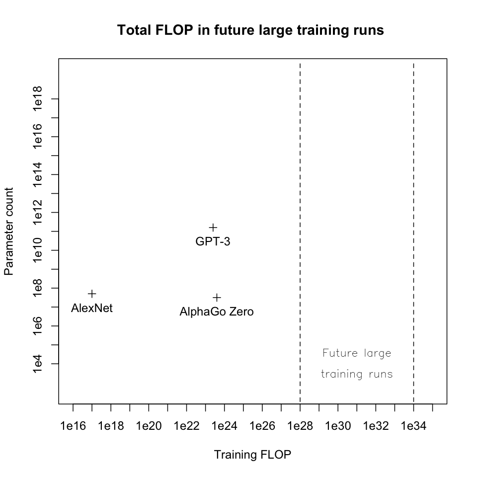
My estimates are summarized in the following chart relating the size of large future training runs, size of trained models produced, and range of possible upper bounds for brain-equivalent capabilities (both axes logarithmic):

The rest of this page builds up this chart over 4 parts:

# Budgets and total FLOP of future training runs: If deep learning continues to attract more funding, we should expect to see the largest training runs use up to 1e28 - 1e34 FLOP (vertical dashed lines in the chart) for projects spending $1B to $100B on training computation (comparable to high-profile physics and space exploration projects on the lower end, and to the Manhattan and Apollo projects on the higher end).

# Model size via scaling laws: Neural scaling laws predict a relationship between total training FLOP and parameter count: for tasks of interest, we should expect trained models to mostly fall in the gray-shaded region in the chart. The top edge of the region corresponds to tasks with frequent, rich feedback (e.g. generative modeling), and the bottom corresponds to tasks with very infrequent, low-quality feedback (e.g. very long-episode reinforcement learning and meta-learning).

# Upper bounds for brain-equivalent capabilities: Using evidence from neuroscience, we can estimate that for any task that the human brain can do in one second or less, a model with ~2e12 - 2e16 parameters (horizontal dotted lines in the chart) should be sufficient to match the brain’s loss, even assuming that the brain has been “trained to convergence” to use its full computational capacity to minimize loss on that specific task. We should expect that for many tasks, models much smaller than this upper bound (with correspondingly lower training costs) will be sufficient.

I think it’s a reasonable bet that replicating the brain’s one-second capabilities is enough to capture a full cognitive “step” that can be applied repeatedly to recurrent state and new inputs in order to put together longer chains of reasoning and planning. Note that the one-second limit does not put any restriction on feedback delays; one-second chunks of brain activity could be optimized to be useful in arbitrarily long chains of activity (as in recurrent models, reinforcement learning, or meta-learning).

# Training data requirements: Neural scaling laws predict that reaching my estimated brain upper bounds would require 1e12 - 1e26 data points. GPT-3 was trained on 3e11 tokens, so this is a big increase; on the other hand, we should expect many tasks to have much lower data requirements than these upper bounds, and 3e11 tokens of text is only ~400GB. Training data could also come from simulation (a small computational expense compared to running the model) or self-play or multi-agent training (at greater computational expense). These estimates don’t appear in the chart.

All of these estimates assume that there are no significant algorithmic or methodological improvements in the next 20-50 years (beyond the work required to train larger models); in reality, these advances could significantly reduce training computation or data requirements.

Budgets and total FLOP of future training runs

Budgets: As of 2020, the largest publicly-documented training runs (GPT-3, AlphaGo Zero, and AlphaStar) each had compute costs in the low millions of dollars (main source: Cotra 2020, supplement).

Computer science has historically not been bottlenecked on expensive experiments, so these costs seem high. But compared to other fields like physics and space exploration, a $1M experimental budget is not especially large: for example, launching a satellite costs $10M to $500M, a Mars lander costs $1B to $3B, and the Large Hadron Collider costs $1B per year to run. If deep learning evolves into a “costly experiment” field, we could expect budgets for the largest training runs to increase gradually to the order of $1B.

On the higher end, deep learning may become a critical factor in international competition. In this case, the largest deep learning research programs could be similar to the Manhattan and Apollo projects, national efforts that cost about 1% of GDP per year for a few years. Scaled to fit to 2020 GDP, Manhattan and Apollo would have annual budgets of around $60B and $140B, respectively, so we might expect an equivalent deep learning megaproject to spend on the order of $10B - $100B on each of a few large training runs per year. As GDP goes up, we should expect these budgets to grow faster than inflation, but I don’t want to get into GDP forecasting for this rough estimate.

(Another reason to take these higher-end budgets seriously, or to think that even higher budgets are plausible, is the already high and fast-growing revenue of technology companies; for example, Google’s annual revenue is already at ~$180B, and it’s easy to imagine that tech companies will have huge amounts of money to work with over the next 20-50 years. If these companies view large training runs as critical to their future success, spending the equivalent of 2020’s revenue in 2030 or 2040 on a key project may seem like a reasonable cost.)

Based on these benchmarks, my order-of-magnitude estimate of the compute budget for future large training runs ranges from $1B to $100B.

FLOP per dollar: The final training runs of GPT-3, AlphaGo Zero, and AlphaStar were able to purchase computation at a price of about 1e17 FLOP per dollar (main source: Cotra 2020, supplement).

It seems likely that the kind of computation used in deep learning will become cheaper over the next few decades, but exactly how much cheaper depends on a huge number of factors across areas ranging from R&D progress to supply chains to general economic growth. So, I’ll give a rough estimate of how FLOP per dollar (FLOP/$) will grow over the next few decades by looking at historical trends.

Like many things in computing, FLOP/$ has historically followed an exponential growth curve. Looking at a few datasets summarized in Trends in the cost of computing (AI Impacts), FLOP per dollar has increased by around 10x every 5-10 years between about 1970 and 2010. I looked more closely at two data points, which fit the higher trend of 10x growth every 5 years (for a total factor of 1e11 over the last 55 years):

The CDC 6600, released in 1964, was one of the earliest transistorized supercomputers. It could perform about 3e6 FLOP/s and cost ~$20M in 2020 dollars, for a performance/cost ratio of about 1e-1 FLOP/s per dollar. (It would be cleaner to use the first transistorized supercomputer, the 1961 IBM 7030 Stretch, as a data-point. I’m skipping to the CDC 6600 because it appears there was some confusion over the 7030’s actual vs advertised speed, its price was quickly cut in half to try to boost sales, and then it was discontinued after only nine sales. The calculations look like they would work out about the same for either computer.)
The NVIDIA Tesla V100 GPU (2020) can perform 1e14 FLOP/s and costs ~$10k, for a performance/cost ratio of 1e10 FLOP/s per dollar.

The trend in general-purpose FLOP per dollar seems more likely to slow down than to speed up, since a lot of low-hanging fruit has already been plucked and some Moore’s-law-like patterns have begun to level off. However, if deep learning continues to show good results, companies will spend a lot of effort looking for ways to continue to lower prices for training-specific computation, and they may succeed: for example, there may be gains from deep-learning-specific hardware, improvements in large-scale computing architecture, increased demand leading to economies of scale in production, and new hardware ideas (e.g. optical computing).

Based on these considerations, my order-of-magnitude estimate for growth in training FLOP per dollar covers a fairly wide range:

On the lower end, 100x improvement over current FLOP/$ (since we don’t yet seem to have hit sharply diminishing returns, and since we could plausibly see this kind of improvement without much progress via cost decreases on existing technology).
On the higher end, a growth rate around 10x every 10 years, leveling off after about half again as much improvement as we’ve seen since 1964 (on a logarithmic scale) – that is, a total growth factor of 1e5 to 1e6 over the next 50 years.

This would take prices from 1e17 FLOP/$ in 2020 gradually up to 1e19 - 1e23 FLOP/$. To me, this looks like a fairly conservative estimate – I think it’s reasonable to argue that I should include a third, even higher tier of growth to account for scenarios where deep learning hardware comes to be seen as a key strategic interest of major governments and companies, driving investment and progress significantly above historical levels, and possibly producing breakthroughs that move hardware efficiency significantly closer to the theoretical physical limits of computing. I didn’t quickly see a good way to model this possibility, so instead I’ll just include this caveat that the “higher end” of my estimate doesn’t look like a solid upper bound.

Combining these prices with my budget estimates, the largest future training runs I’m considering could use up to 1e28 - 1e34 FLOP:

Model size via scaling laws

Scaling Laws for Neural Language Models (Kaplan and McCandlish et al. 2020) studies the relationship between performance, model size, training data, and training computation for language-modeling Transformers. They propose a law for the predicted loss of a model with $N$ parameters trained on $D$ data points, with experimentally-determined constants $\alpha_N$ , $\alpha_D$ , $N_c$ , and $D_c$ (equation 1.5, pages 5 and 10):

$L(N, D) = \left[ \left(\frac{N_c}{N}\right)^{\frac{\alpha_N}{\alpha_D}} + \frac{D_c}{D} \right]^{\alpha_D}$

This predicts that loss falls with diminishing returns as parameter count and dataset size increase, approximately following the power laws $N^{-\alpha_N}$ and $D^{-\alpha_D}$ . In our current state of knowledge, I think it’s a reasonable bet that the scaling behavior of many machine learning tasks will fit laws of roughly this form.

Additional training computation can either be spent to increase the size of the model or to train it on more data. We can use equation 1.5 to predict the size of an “efficiently-trained” model, i.e. a model that minimizes loss for a fixed amount of training computation by optimally balancing model size and training data. See appendix A for my derivation of this equation:

$N \approx \left[FLOP\times\left(\frac{N_c^{\frac{\alpha_N}{\alpha_D}}}{D_c}\right) \left(\frac{\alpha_N}{\alpha_D}\right)\right]^{\frac{1}{1+\frac{\alpha_N}{\alpha_D}}$

As a sanity check, using the constants from Scaling Laws p.11, this equation predicts that with a training budget of 3.14e23, GPT-3 should have 1.27e11 parameters (vs. its actual parameter count of 1.75e11, Language Models are Few-Shot Learners (Brown, Mann, Ryder, and Subbiah et al. 2020) p.46). A reasonably good fit should be expected, since results from Scaling Laws were used to guide GPT-3’s training.

(Scaling Laws proposes and empirically tests another neural scaling law, $L(C)$ , relating loss directly to training computation. I’m using $L(N, D)$ as the basis for my estimates because it looks more likely to me to continue to hold for very large models; for discussion, see pg. 17-18 of Scaling Laws, and pg. 17-19 of Scaling Laws for Autoregressive Generative Modeling (Henighan, Kaplan, and Katz et al. 2020)).

To estimate the size of models produced by future large training runs, we need ranges of constants that we expect to describe the kinds of tasks we’re interested in. I use the following ranges:

Ratio of exponents ( $\alpha_N/\alpha_D$ ): 0.5 - 1. The value found in Scaling Laws is 0.74; I’m choosing the range [0.5, 1] to reflect my expectation that data will generally grow sublinearly in model size.
$N_c$ : 1e13 - 1e16. Doubling $N_c$ doubles the number of parameters needed to reach a given loss. The value found in Scaling Laws is 6.4e13; since general language modeling captures a very broad range of behaviors (see e.g. Language Models are Few-Shot Learners), I’m making the very broad guess that tasks of interest will not have significantly more than 1,000x the parameters-to-loss requirement of language modeling, for an upper bound of $N_c$ = 1e16.
$D_c$ : 1e13 - 1e23. Doubling $D_c$ doubles the number of training data samples needed to reach a given loss. The Scaling Laws value of $D_c$ is 1.8e13, suggesting that $N_c$ and $D_c$ both reflect the complexity of the underlying distribution, so I’ll generally use $D_c \geq N_c$ .

$D_c$ should be larger for tasks where some important feedback is infrequent or low-quality (e.g. meta-learning and RL). Following Forecasting transformative AI with biological anchors, we can get a rough sense of the plausible range of $D_c$ by comparing to the kinds of tasks biological brains evolved to perform. Assuming that a model does 1-10 forward passes per second (on par with human reading speed, reaction time, etc.), 1e5 data points corresponds to ~3-30 hours of experience, and 1e10 data points corresponds to ~30-300 years.

Based on this, I would be surprised to see tasks with $D_c$ >> 1e23, roughly corresponding to a natural language modeling task that reveals only one token worth of information every 1e10 data points.

With these ranges of constants, we can graph predicted parameter count against training FLOP:

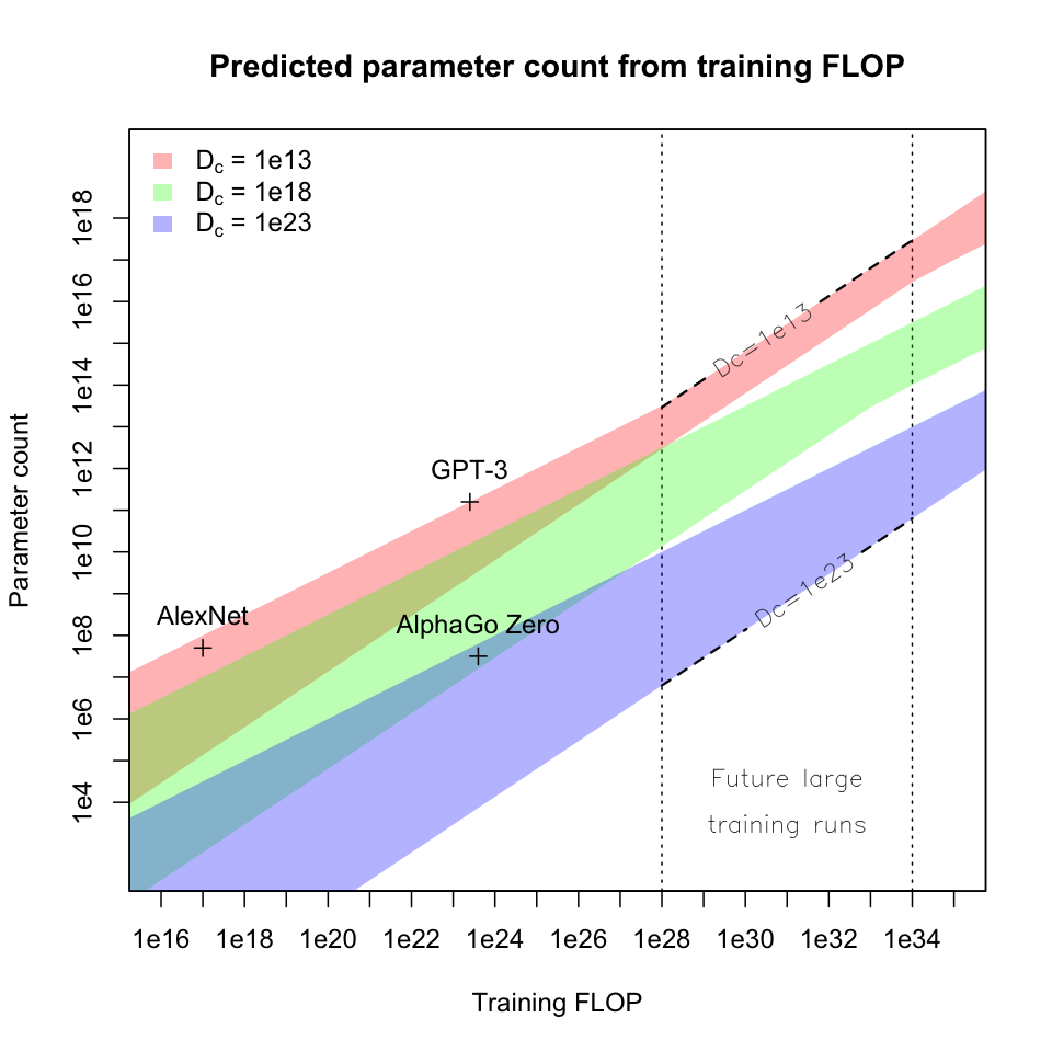
Each band of color corresponds to the set of tasks with a given value of $D_c$ , covering an area that includes all settings of $\alpha_N/\alpha_D$ in [0.5, 1] and all settings of $N_c$ in [1e13, 1e16] (subject to the constraint that $Dc \geq N_c$ ); gaps between bands would be filled by intermediate values of $D_c$ . Vertical dashed lines mark the low and high predicted FLOP of future large training runs from previous sections. Bends in the bands are caused by an interaction between the exponents and multiplicative terms of the underlying scaling laws.

My main conclusions from this exercise are:

For tasks of interest and training runs in the 1e28 - 1e34 training FLOP range, it would be surprising to see efficiently-trained models far outside the region show on the chart with dotted lines, given by $D_c$ = [1e13, 1e23], $N_c$ = 1e13, and $\alpha_N/\alpha_D$ = 0.5.
Within this region, the biggest factors determining model size are training FLOP and “feedback sparsity” $D_c$ ; the top edge of the region corresponds to tasks with frequent, rich feedback (e.g. generative modeling), and the bottom corresponds to tasks with very infrequent, low-quality feedback (e.g. very long-episode reinforcement learning and meta-learning). As $D_c$ varies over 10 orders of magnitude, predicted model sizes vary over about 6.5 orders of magnitude.

Upper bounds for brain-equivalent capabilities

In this section, I’ll give a range of estimated upper bounds on the size a model would need to be in order to be efficiently trained to do (in one forward pass) any task a human brain can do in less than a second. We should expect any specific capability to be reached somewhere below this bound – it seems likely that most tasks use a small fraction of the brain’s total computation, and in fact we have reached human-like capabilities on many tasks with relatively small models (e.g. MNIST, ImageNet, or choosing a competent Go move).

To estimate the 1-full-brain-second-equivalent upper bound, I go through the following steps:

Estimate the size a model would need to be in order to perform 1 brain-second of computation per forward pass;
Assume that the brain’s performance on any task is the same as the performance of a model that does 1-brain-second of computation, trained to convergence on that task;
Calculate the size an efficiently-trained model would need to be in order to match the loss of this 1-brain-sec. per forward pass converged model.

How Much Computational Power Does It Take To Match The Human Brain? (Carlsmith 2020) reviews evidence from neuroscience to estimate the human brain’s computational capacity. The full report has much more detail, but I think the most compelling estimate is that one brain-second of computation is in the ballpark of 1e13 - 1e17 FLOP:

On a per-synapse basis (est. 1e14 - 1e15 synapses receiving spikes every 0.1-1 sec), this would be 1-100 FLOP per spike per synapse.
On a per-neuron basis (est. 1e11 neurons spiking every 0.1-1 sec), this would be 1e2 - 1e6 FLOP per spike.
Other mechanisms seem unlikely to contribute enough computation to significantly change the FLOP/s estimate, even if they play important roles.

Assuming that a model performs around 10 FLOP per parameter per forward pass, a model that does one brain-second of computation per forward pass would need 1e12 - 1e16 parameters.

Brain evolution is dissimilar from efficient training in many ways. On the one hand, it seems highly implausible that each synapse has been independently optimized by evolution – given that the human genome is only ~7.5e8 bytes, it seems very unlikely that genetic or epigenetic mechanisms could even carry the necessary information to make the “settings” of each of 1e14 synapses individually heritable. This could mean that a model many orders of magnitude smaller than the brain could achieve similar performance. On the other hand, brains don’t lose any fitness for taking a long time to evolve, but do pay a fitness cost per additional neuron and operation (in calories, weight, and size). This could mean that a human brain is best approximated as a converged model, and that we should expect an efficiently-trained model with the same loss to be somewhat larger and less-optimized.

In order to push this estimate towards an upper bound on how large efficiently trained models will need to be, I’ll follow the second point, and model the human brain as a converged model of 1e12 - 1e16 parameters. (This bakes in the conservative, but highly unlikely, assumption that the brain is trained to convergence on all tasks of interest.)

From Scaling Laws, we can derive a relationship between the sizes of efficiently-trained and converged models that get the same loss on the same task (see appendix B for the derivation):

$L_{\textit{efficient}}(N) = L\left(N / \left(1+\frac{\alpha_N}{\alpha_D} \right)^{\frac{\alpha_D}{\alpha_N}},\infty\right)$

For my estimated range of $\alpha_N/\alpha_D$ = [0.5, 1], an efficiently-trained model needs to be 2x - 2.25x larger than a converged model in order to match its loss; for this estimate, I’ll take the median value of ~2.13, though this ratio is so small compared to other factors that this choice doesn’t matter much.

This gives an estimated upper bound of ~2e12 - 2e16 on the size an efficiently-trained model would need to be in order to replicate a human brain’s 1-second capabilities:

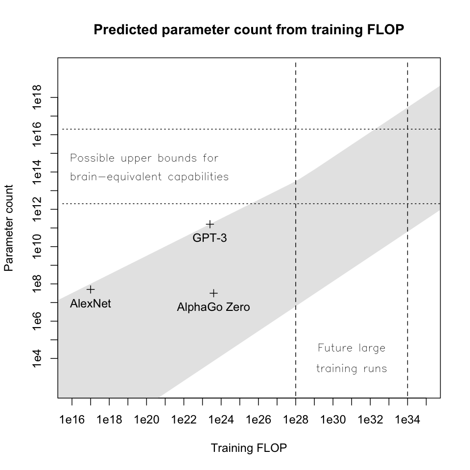
This section is especially rough. A few of my largest reservations are:

This estimate ignores the fact that we continue to see large increases in model performance from architectural improvements, but this kind of improvement seems likely to be one of the most important factors that could affect the performance of models vs. brains over a 20-50 year timeframe. Even for a Fermi estimate, this is a large omission.
~2e12 parameters is already very close to GPT-3’s 1.75e11 parameters. This could mean that there’s something wrong with my estimate or the overall framework of this report, or it could mean that we’re surprisingly close to the computational requirements for replicating all of the human brain’s one-second abilities on dense-feedback tasks like generative modeling. (I think the latter is not completely implausible; it’s not clear to me that a human could do orders of magnitude better than GPT-3 at pure next-token prediction, and improving GPT-3’s long-term coherence would require increasingly sparse feedback, increasing the cost of training significantly without increasing model size much.)
The form of the efficiently-trained vs. converged model size equation implies that the size ratio between efficiently-trained and converged models with the same loss will never get very large: in the limits of $\alpha_N/\alpha_D\to 0$ and $\alpha_N/\alpha_D\to\infty$ , the ratio is bounded by 1 and 2.718 (= $e$ ), respectively. This result surprises me, and makes me wonder whether there are some deeper things about training dynamics that I’m not understanding (that either make this result unsurprising, or show that it is false).

Training data requirements

The same neural scaling laws I’ve been using throughout this report can be used to derive equations relating training dataset size to training FLOP and parameter count; these derivations can be found in appendix C and the first part of appendix A, respectively. These equations give the following graphs:

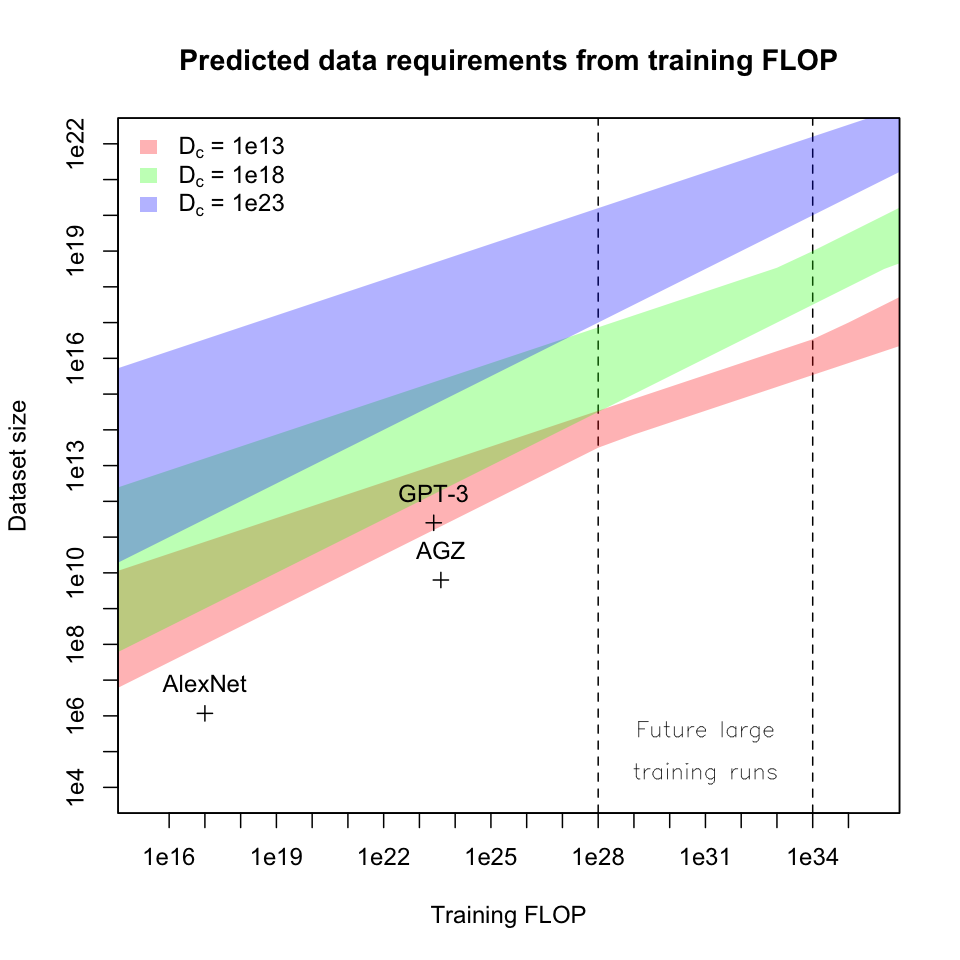
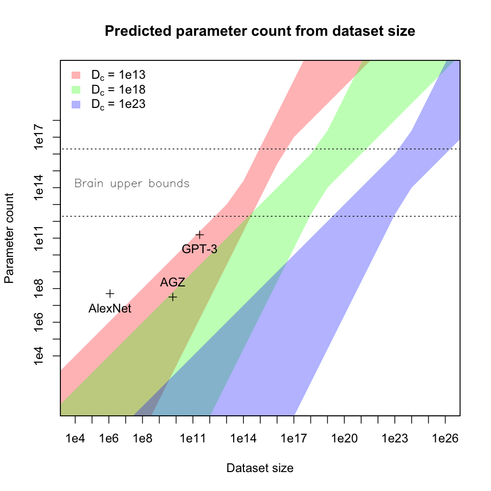
These graphs again show that multiplicative constants in the scaling laws are large enough that the transition to “in the limit” behavior is only starting to take hold in the 1e28 - 1e34 FLOP range, giving the bands a bendy shape. Gaps between bands would be filled by intermediate values of $D_c$ .

I’m not sure what to make of AlexNet on these charts – my best guess is that it’s old enough to not reflect current best practices about balancing data, computation, and parameters, but I haven’t looked into it. AlphaGo Zero is more interesting: I think its position below the red band in the first graph reflects the potential for “data points” to be much more expensive in self-play or multi-agent training setups.

As expected, larger models and training runs require much more data; training runs in the 1e28 - 1e34 FLOP range would require 1e13 - 1e22 data points, and reaching my estimated brain upper bounds would require 1e12 - 1e26 data points. These ranges are ~10x - 1e15x more training data than GPT-3.

I think it’s plausible that we’ll be able to pay these costs, especially on a 20-50 year timeframe:

First, GPT-3’s 3e11 tokens only comes to ~400GB of data, so we’re not approaching any natural limit on available training data.
Second, training data could come from simulation (a small computational expense compared to running the model) or self-play / multi-agent training (at greater computational expense).
Third, we should expect many capabilities to have much lower data requirements than this upper bound.

As a side note, these estimates strongly suggest that in the kinds of large training runs I’ve described here, only a tiny fraction of training data can involve direct human labeling, supervision, or feedback.

Appendices

A: Derivation of parameters vs. training FLOP equation

I’ll approximate the computational cost of training as the cost of running the model on each data point: (N parameters) * (1 forward pass per data point D) * (a small number of FLOP per parameter per forward pass) ~= total FLOP on the order of $N \times D$ .

For a particular training run defined by its model size and dataset size $(N, D)$ , there is a set of training runs of equivalent cost given by $(N/x, xD)$ , where x takes on any value greater than zero. We can find the predicted loss of any of these training runs using equation 1.5:

$\begin{aligned} L(N/x, xD) &= \left[ \left(\frac{N_c}{N/x}\right)^{\frac{\alpha_N}{\alpha_D}} + \frac{D_c}{xD}\right]^{\alpha_D} \\ &= \left[ \left(\frac{N_c}{N}\right)^{\frac{\alpha_N}{\alpha_D}}x^{\frac{\alpha_N}{\alpha_D}} + \frac{D_c}{D}x^{-1}\right]^{\alpha_D} \\ \end{aligned}$

Efficient training balances parameter count and dataset size to minimize loss within a set of cost-equivalent training runs. So, we want to know what relationship between D and N causes $L(N/x, xD)$ to be minimized when x = 1. Since we’re interested in the minima of $L(N/x, xD)$ , we can drop the outermost exponent $\alpha_D$ . We then take the derivative with respect to x:

$\begin{aligned} \frac{d}{dx}L &= \frac{\alpha_N}{\alpha_D}\left(\frac{N_c}{N}\right)^{\frac{\alpha_N}{\alpha_D}}x^{\frac{\alpha_N}{\alpha_D}-1} - \frac{D_c}{D}x^{-2} \\ \end{aligned}$

Now we set x = 1 and $dL/dx = 0$ and solve for D:

$\begin{aligned} 0 &= \frac{\alpha_N}{\alpha_D}\left(\frac{N_c}{N}\right)^{\frac{\alpha_N}{\alpha_D}} - \frac{D_c}{D} \\ \frac{D_c}{D} &= \frac{\alpha_N}{\alpha_D}\left(\frac{N_c}{N}\right)^{\frac{\alpha_N}{\alpha_D}}\\ D &= D_c\frac{\alpha_D}{\alpha_N}\left(\frac{N}{N_c}\right)^{\frac{\alpha_N}{\alpha_D}}\\ D &= \left(\frac{D_c}{N_c^{\frac{\alpha_N}{\alpha_D}}}\right) \left(\frac{\alpha_D}{\alpha_N}\right) N^{\frac{\alpha_N}{\alpha_D}} \end{aligned}$

This last line is a scaling law relating dataset size D to parameter count N; as expected, D is proportional to $N^{\alpha_N/\alpha_D}$ . Now we can substitute this expression into the equation for total training FLOP and solve for N, to get an equation relating parameter count to total training FLOP:

$\begin{aligned} \text{FLOP} &\approx ND \\ &\approx \left(\frac{D_c}{N_c^{\frac{\alpha_N}{\alpha_D}}}\right) \left(\frac{\alpha_D}{\alpha_N}\right) N^{1+\frac{\alpha_N}{\alpha_D}} \\ N^{1+\frac{\alpha_N}{\alpha_D}} &\approx \text{FLOP}\times \left(\frac{N_c^{\frac{\alpha_N}{\alpha_D}}}{D_c}\right) \left(\frac{\alpha_N}{\alpha_D}\right)\\ N &\approx \left[\text{FLOP}\times \left(\frac{N_c^{\frac{\alpha_N}{\alpha_D}}}{D_c}\right) \left(\frac{\alpha_N}{\alpha_D}\right)\right]^{\frac{1}{1+\frac{\alpha_N}{\alpha_D}}}\\ \end{aligned}$

B: Derivation of converged vs. efficiently-trained models equation

In this section, I derive a relationship between the sizes of efficiently-trained and converged models that get the same loss on the same task. A convenient place to start is an intermediate step from appendix A. During efficient training, we have:

$\frac{D_c}{D} = \frac{\alpha_N}{\alpha_D}\left(\frac{N_c}{N}\right)^{\frac{\alpha_N}{\alpha_D}}$

We can substitute this into the $L(N, D)$ scaling law to get a formula for $L_\textit{efficient}(N)$ , the loss of an efficiently-trained model with N parameters:

$\begin{aligned} L(N, D) &= \left[ \left(\frac{N_c}{N}\right)^{\frac{\alpha_N}{\alpha_D}} + \frac{D_c}{D} \right]^{\alpha_D} \\ L_\textit{efficient}(N) &= \left[ \left(\frac{N_c}{N}\right)^{\frac{\alpha_N}{\alpha_D}} + \frac{\alpha_N}{\alpha_D}\left(\frac{N_c}{N}\right)^{\frac{\alpha_N}{\alpha_D}} \right]^{\alpha_D} \\ &= \left[ \left(1+\frac{\alpha_N}{\alpha_D} \right)\left(\frac{N_c}{N}\right)^{\frac{\alpha_N}{\alpha_D}} \right]^{\alpha_D} \\ &= \left(1+\frac{\alpha_N}{\alpha_D} \right)^{\alpha_D} \left(\frac{N_c}{N}\right)^{\alpha_N} \\ &= \left(\frac{N_c}{N/\left(1+\frac{\alpha_N}{\alpha_D} \right)^{\alpha_D/\alpha_N}}\right)^{\alpha_N} \\ \end{aligned}$

This expression has the same form as the scaling law for converged models (equation 1.1, page 4 of Scaling Laws for Neural Language Models):

$L(N, \infty) = \left(\frac{N_c}{N}\right)^{\alpha_N}$

This gives us the relationship between the sizes of efficiently-trained and converged models that get the same loss:

$L_{\textit{efficient}}(N) = L\left(N / \left(1+\frac{\alpha_N}{\alpha_D} \right)^{\frac{\alpha_D}{\alpha_N}},\infty\right)$

As $\alpha_N/\alpha_D$ approaches 0, I would have expected efficient training to call for arbitrarily large models trained on arbitrarily small datasets, causing the size ratio between efficiently-trained and converged models to get arbitrarily large (until model size and dataset size get so extreme that scaling laws no longer apply). However, as $\alpha_N/\alpha_D$ approaches 0, the factor $(1 + \alpha_N/\alpha_D)^{\alpha_D/\alpha_N}$ approaches an upper limit of $e$ ~= 2.718, implying that an efficiently-trained model is at most $e$ times larger than a converged model with the same loss.

Since I expect values of $\alpha_N/\alpha_D$ to be not much smaller than 0.5, I don’t think this will have practical implications, but I still find this effect surprising.

C: Derivation of dataset size vs. training FLOP equation

This derivation starts with the relationship between dataset size D and parameter count N during efficient training (appendix A):

$D = D_c\frac{\alpha_D}{\alpha_N}\left(\frac{N}{N_c}\right)^{\frac{\alpha_N}{\alpha_D}}$

Solving for N, we have:

$\begin{aligned} D &= \left(\frac{D_c}{N_c^{\frac{\alpha_N}{\alpha_D}}}\right) \left(\frac{\alpha_D}{\alpha_N}\right) N^{\frac{\alpha_N}{\alpha_D}} \\ N^{\frac{\alpha_N}{\alpha_D}} &= \left(\frac{N_c^{\frac{\alpha_N}{\alpha_D}}}{D_c}\right) \left(\frac{\alpha_N}{\alpha_D}\right) D\\ N &= \left(\frac{N_c}{D_c^{\frac{\alpha_D}{\alpha_N}}}\right) \left(\frac{\alpha_N}{\alpha_D}\right)^{\frac{\alpha_D}{\alpha_N}} D^{\frac{\alpha_D}{\alpha_N}} \end{aligned}$

Now we can substitute this expression into the equation for total training FLOP and solve for D, to get an equation relating dataset size to total training FLOP:

$\begin{aligned} FLOP &\approx ND \\ FLOP &\approx \left(\frac{N_c}{D_c^{\frac{\alpha_D}{\alpha_N}}}\right) \left(\frac{\alpha_N}{\alpha_D}\right)^{\frac{\alpha_D}{\alpha_N}} D^{1+\frac{\alpha_D}{\alpha_N}} \\ D^{1+\frac{\alpha_D}{\alpha_N}} &\approx FLOP\times \left(\frac{D_c^{\frac{\alpha_D}{\alpha_N}}}{N_c}\right) \left(\frac{\alpha_D}{\alpha_N}\right)^{\frac{\alpha_D}{\alpha_N}}\\ D &\approx \left[FLOP\times \left(\frac{D_c^{\frac{\alpha_D}{\alpha_N}}}{N_c}\right) \left(\frac{\alpha_D}{\alpha_N}\right)^{\frac{\alpha_D}{\alpha_N}}\right]^{\frac{1}{1+\frac{\alpha_D}{\alpha_N}}} \end{align*}$

Applications of high-capability models

Global risk from deep learning